Week 9: ggplot2 Basics

PPOL 6805: GIS for Spatial Data Science

R Coding Workshop for GIS: 7th Meeting

Outline

• Organize and save analysis results
• ggplot

Initialize a ggplot object

To create a ggplot object, we need…

Components:

• data
• mapping
• geometry layer

Steps:

1. Prepare your data (often in the structure of a dataframe object)
2. Think about the variable(s) that you’re interested in and what type of geometry (marks: point/line/polygon) might best help you understand their distribution or relationship.
3. Specify them using the grammar of graphics –map the variables to corresponding aesthetic or spatial properties of the geometry (color/size/position x, y)

ggplot(): data being the first argument

book_df <- read_csv('data/book-df-us-main.csv')

Rows: 47 Columns: 25
── Column specification ────────────────────────────────────────────────────────
Delimiter: ","
chr  (2): state, division_str
dbl (23): division_code, political_value_index, median_income, hs_grad_rate,...

ℹ Use `spec()` to retrieve the full column specification for this data.
ℹ Specify the column types or set `show_col_types = FALSE` to quiet this message.

book_df |> glimpse()

Rows: 47
Columns: 25
$ state                 <chr> "WY", "PA", "OH", "NM", "MD", "RI", "OR", "WI", …
$ division_code         <dbl> 8, 2, 3, 8, 5, 1, 9, 3, 4, 8, 5, 2, 7, 4, 4, 8, …
$ division_str          <chr> "Mountain", "Middle Atlantic", "East North Centr…
$ political_value_index <dbl> -19.7, 2.0, -0.7, 2.4, 8.5, 11.2, 4.0, 2.4, -10.…
$ median_income         <dbl> 4081.5, 4218.0, 2469.0, -2401.5, 19404.5, 8141.0…
$ hs_grad_rate          <dbl> 8.3380421, 2.3380421, 3.4380421, -0.6619579, 4.2…
$ college_grad_rate     <dbl> -2.1237299, -1.6237299, -2.9237299, -0.5237299, …
$ challenge_count       <dbl> 4, 148, 29, 3, 5, 3, 118, 10, 6, NA, 13, 25, 5, …
$ explicit_count        <dbl> 1, 15, 13, 1, 2, 3, 26, 5, 2, NA, 4, 7, 1, 6, 1,…
$ antifamily_count      <dbl> 0, 2, 5, 0, 1, 0, 1, 0, 0, NA, 1, 2, 0, 0, 0, 0,…
$ occult_count          <dbl> 0, 3, 2, 0, 0, 0, 3, 1, 0, NA, 0, 1, 1, 1, 0, 0,…
$ language_count        <dbl> 0, 16, 14, 1, 3, 2, 14, 3, 2, NA, 7, 9, 3, 5, 1,…
$ lgbtq_count           <dbl> 1, 5, 1, 0, 2, 0, 10, 1, 0, NA, 3, 3, 0, 0, 0, 0…
$ violent_count         <dbl> 1, 6, 2, 0, 2, 0, 19, 2, 1, NA, 3, 3, 1, 3, 1, 0…
$ removed_count         <dbl> 1, 11, 10, 2, 0, 1, 5, 3, 2, NA, 4, 11, 0, 10, 0…
$ removed_pct           <dbl> 25.000000, 7.432432, 34.482759, 66.666667, 0.000…
$ POPU_LSA              <dbl> 544270, 12054201, 11551941, 1588981, 5633514, 14…
$ POPU_ST               <dbl> 544270, 12284183, 11551941, 2009671, 5618344, 10…
$ CENTLIB               <dbl> 23, 451, 240, 91, 15, 47, 122, 378, 80, 19, 61, …
$ BRANLIB               <dbl> 53, 183, 480, 27, 169, 26, 94, 82, 10, 67, 331, …
$ BKMOB                 <dbl> 2, 29, 58, 1, 18, 2, 8, 6, 12, 4, 17, 6, 1, 4, 7…
$ BKVOL                 <dbl> 2497545, 27790282, 45224425, 4518130, 13954140, …
$ LIBRARIA              <dbl> 189.16, 1445.81, 2725.65, 290.37, 1297.29, 232.1…
$ VISITS                <dbl> 3872783, 47188171, 88255852, 8324986, 33662473, …
$ REGBOR                <dbl> 383126, 5549200, 8767349, 1140637, 3271760, 5747…

Plotting the distribution of a single variable

• view()

# book_df |> view()

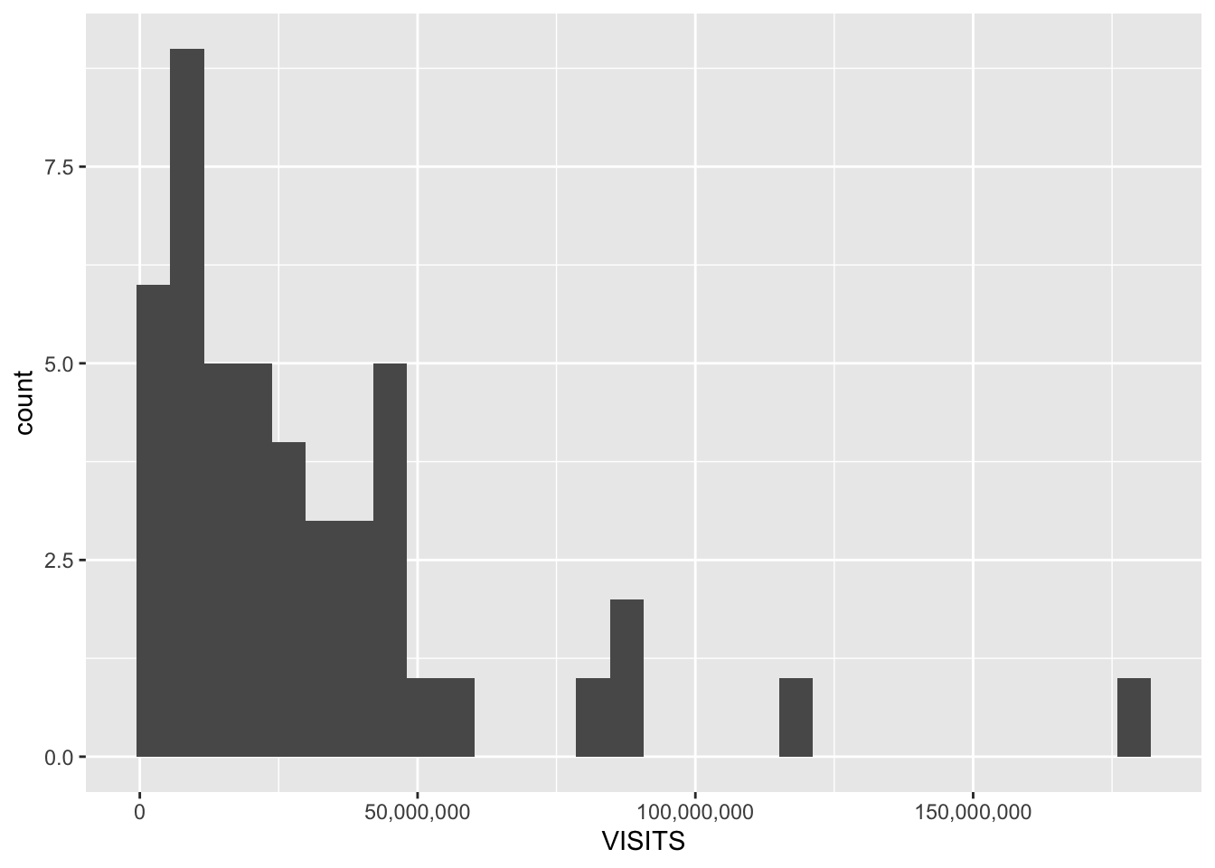
• layer geom_histogram(): for a numeric variable

book_df |>
  ggplot(mapping = aes(VISITS)) +
  geom_histogram() +
  scale_x_continuous(labels = comma)

`stat_bin()` using `bins = 30`. Pick better value `binwidth`.

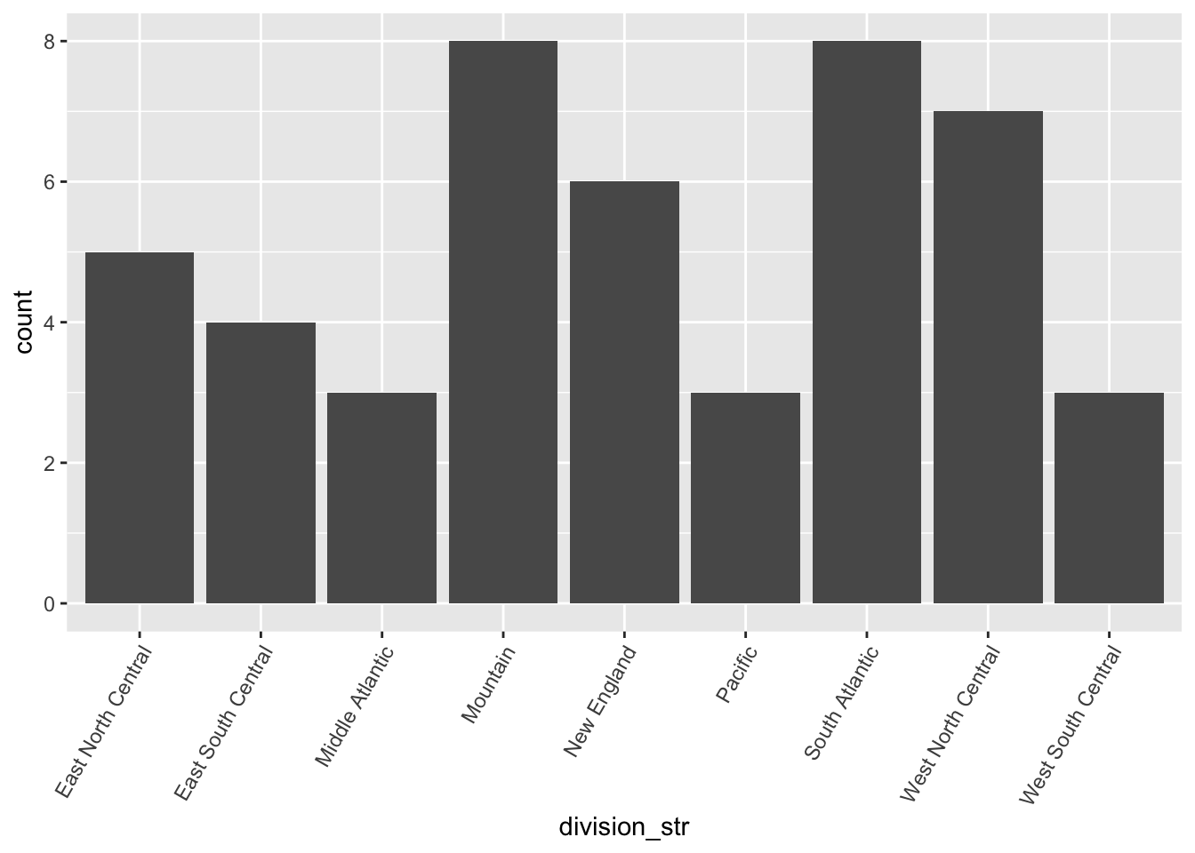
• layer geom_bar(): for a categorical variable

book_df |>
    ggplot(aes(x = division_str)) +
    geom_bar() +
    guides(x = guide_axis(angle = 60))

Distribution

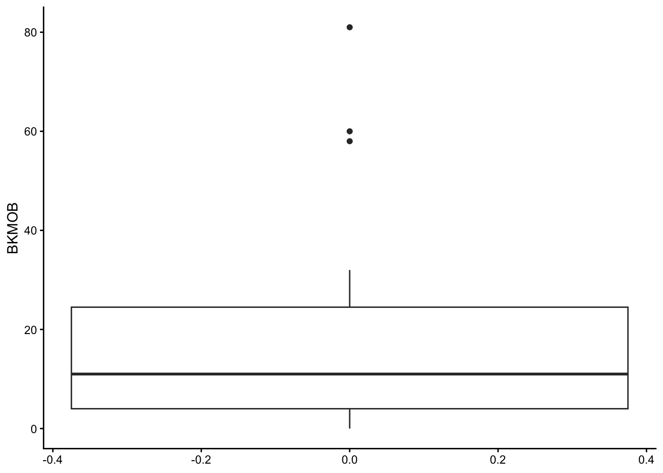
geom_boxplot()

decompose the elements of ggplot specification

• map variable name to aes attribute
• add geometry layer with + sign
• extra: change the theme layer to classic

book_df |>
  ggplot(mapping = aes(y = BKMOB)) +
  geom_boxplot() +
  theme_classic()

Association

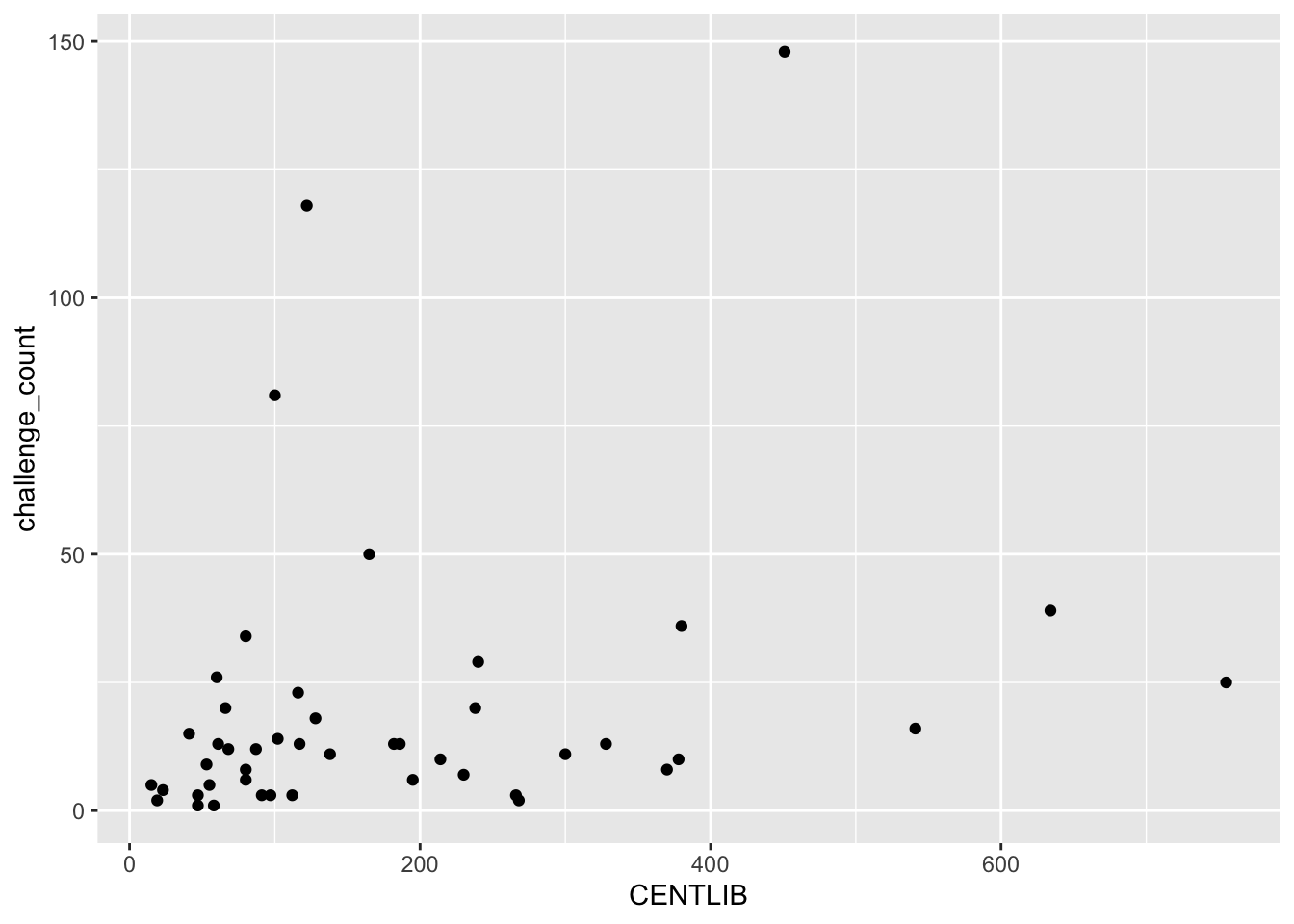
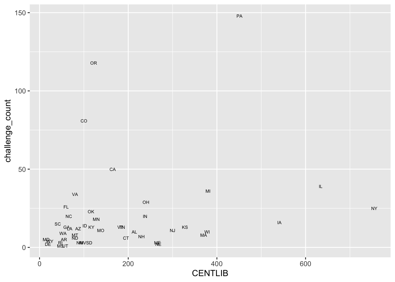
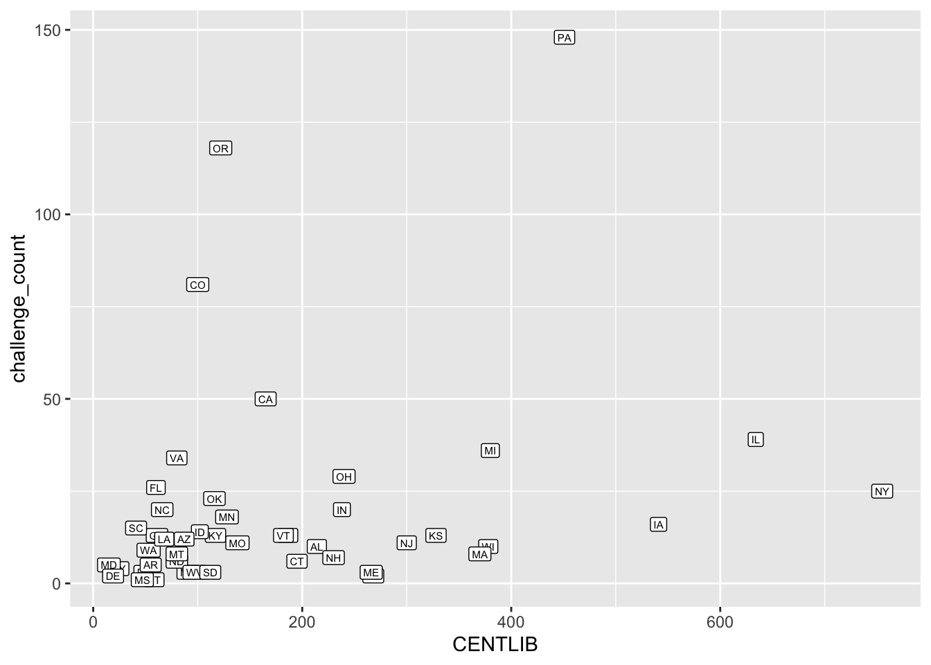
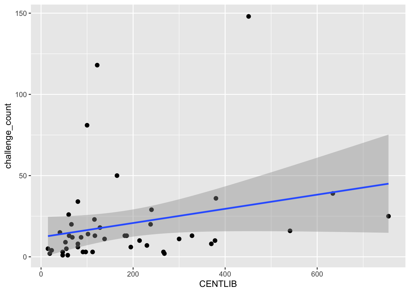
• geom_point(), geom_text(), geom_label(): two variable, using points to mark position

bk_df <- read_csv('data/book-df-us-main.csv')

Rows: 47 Columns: 25
── Column specification ────────────────────────────────────────────────────────
Delimiter: ","
chr  (2): state, division_str
dbl (23): division_code, political_value_index, median_income, hs_grad_rate,...

ℹ Use `spec()` to retrieve the full column specification for this data.
ℹ Specify the column types or set `show_col_types = FALSE` to quiet this message.

bk_df |>
    ggplot(aes(x = CENTLIB, y = challenge_count, label = state)) +
    geom_point()

Warning: Removed 1 row containing missing values or values outside the scale range
(`geom_point()`).

bk_df |>
    ggplot(aes(x = CENTLIB, y = challenge_count, label = state)) +
    geom_text(size = 2)

Warning: Removed 1 row containing missing values or values outside the scale range
(`geom_text()`).

bk_df |>
    ggplot(aes(x = CENTLIB, y = challenge_count, label = state)) +
    geom_label(size = 2)

Warning: Removed 1 row containing missing values or values outside the scale range
(`geom_label()`).

bk_df |>
    ggplot(aes(x = CENTLIB, y = challenge_count, label = state)) +
    geom_point(size = 2) +
    geom_smooth(method = 'lm')

`geom_smooth()` using formula = 'y ~ x'

Warning: Removed 1 row containing non-finite outside the scale range
(`stat_smooth()`).

Warning: The following aesthetics were dropped during statistical transformation: label.
ℹ This can happen when ggplot fails to infer the correct grouping structure in
  the data.
ℹ Did you forget to specify a `group` aesthetic or to convert a numerical
  variable into a factor?

Warning: Removed 1 row containing missing values or values outside the scale range
(`geom_point()`).

Comparison

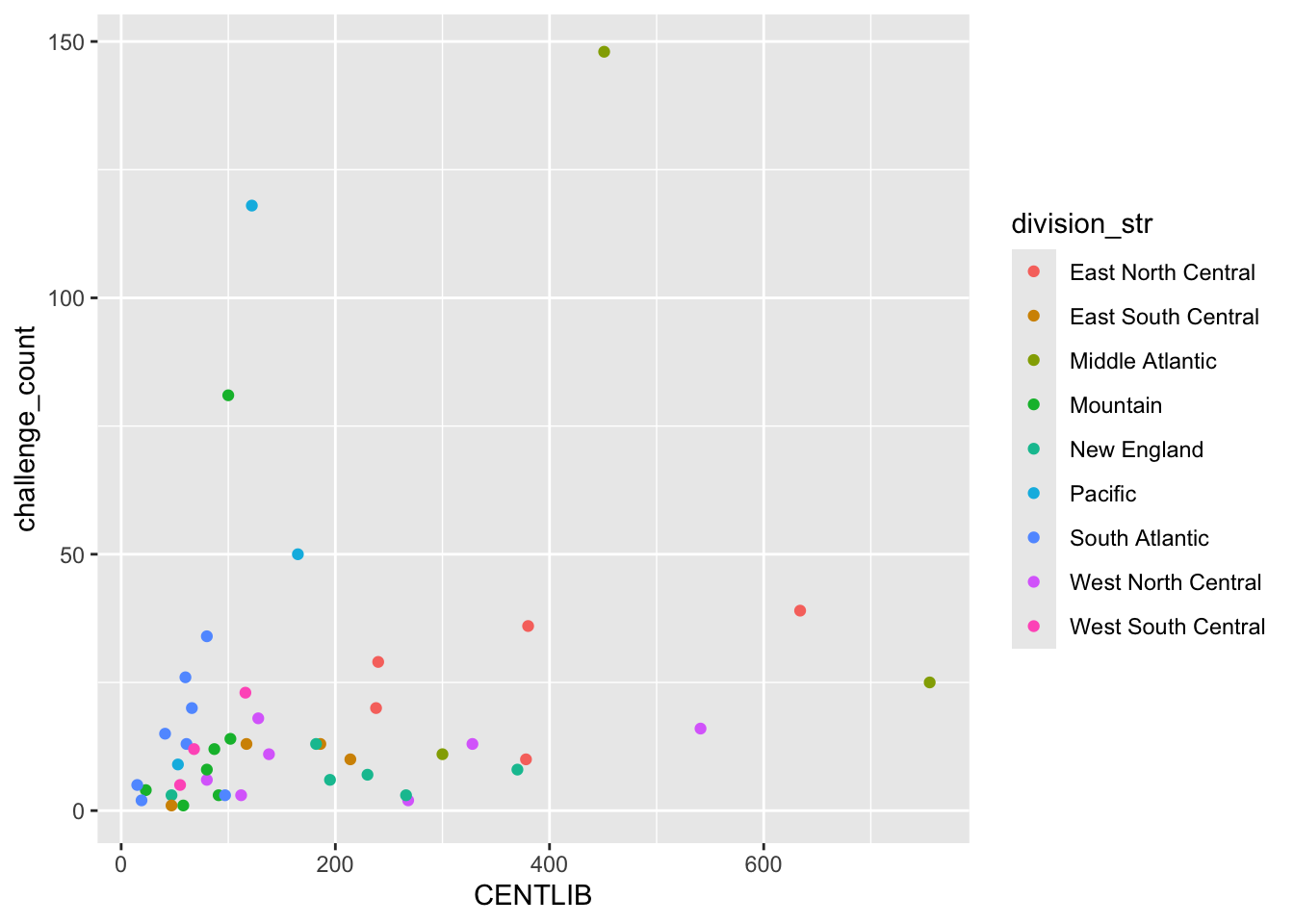
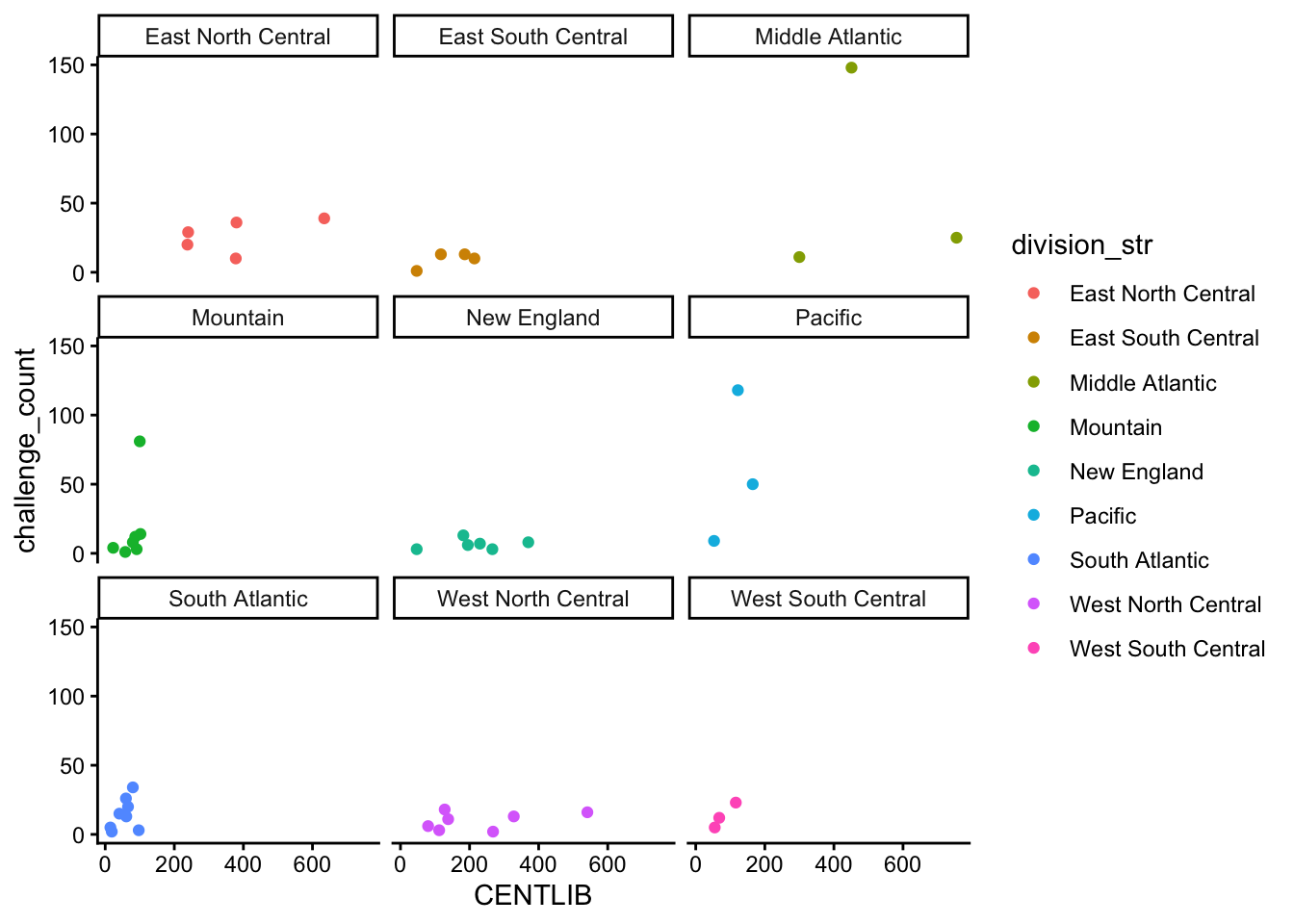
• Add a z variable: color, size, facet_wrap()

bk_df |>
    ggplot(aes(x = CENTLIB, y = challenge_count, color = division_str)) +
    geom_point()

Warning: Removed 1 row containing missing values or values outside the scale range
(`geom_point()`).

bk_df |>
    ggplot(aes(x = CENTLIB, y = challenge_count, color = division_str)) +
    geom_point() +
    facet_wrap(~division_str) +
    theme_classic()

Warning: Removed 1 row containing missing values or values outside the scale range
(`geom_point()`).

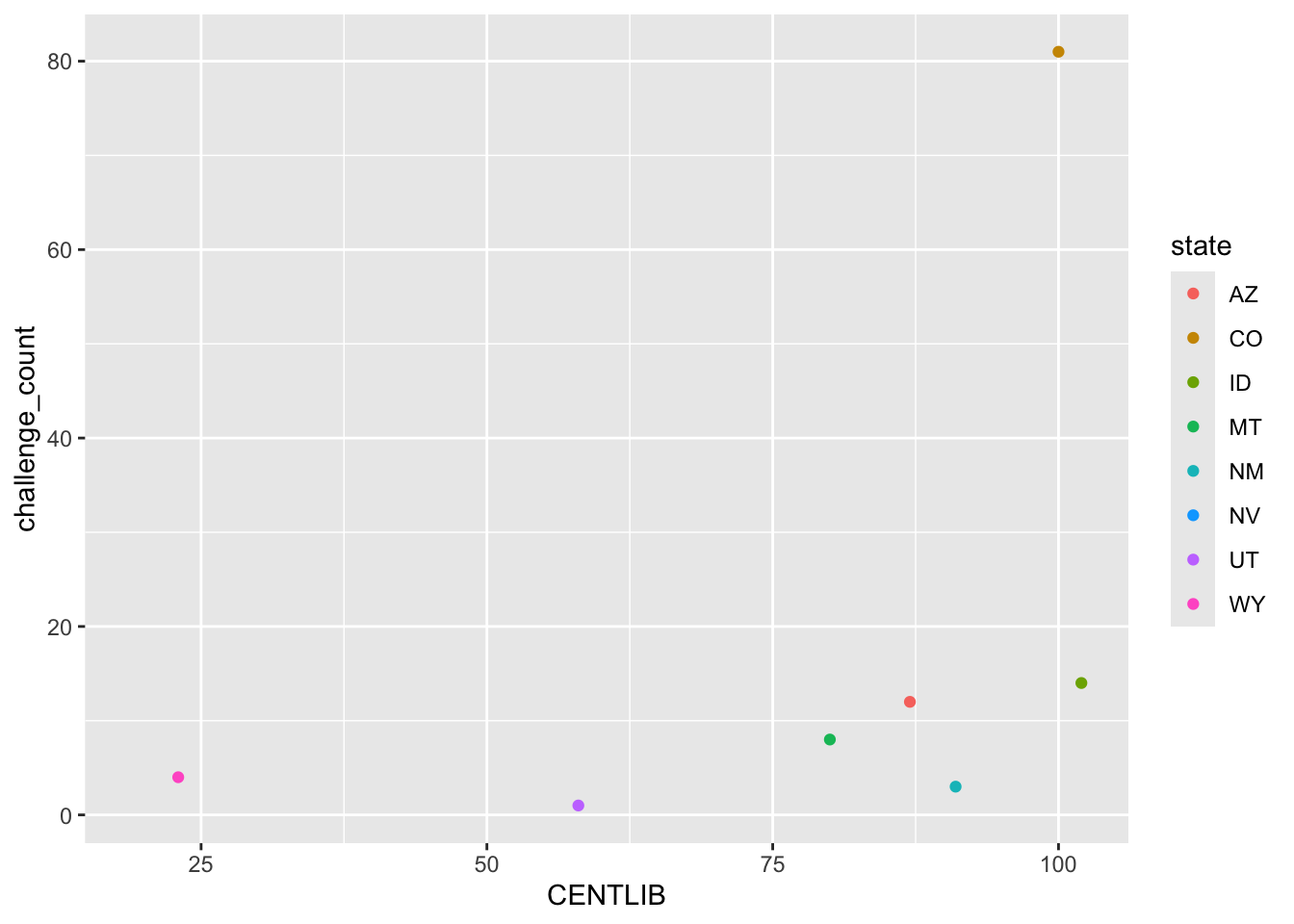
bk_df |>
  filter(division_str == 'Mountain') |>
  ggplot(aes(x = CENTLIB, y = challenge_count, color = state)) +
  geom_point()

Warning: Removed 1 row containing missing values or values outside the scale range
(`geom_point()`).

ggplot for sf

• geom_sf()

library(tigris)

To enable caching of data, set `options(tigris_use_cache = TRUE)`
in your R script or .Rprofile.

Attaching package: 'tigris'

The following object is masked from 'package:terra':

    blocks

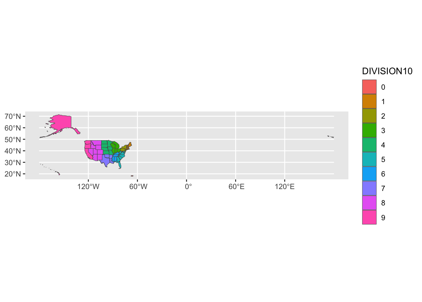
states_sf <- states(year = 2010, progress_bar = FALSE)
# states_sf

states_sf |>
  ggplot() +
  geom_sf(aes(fill = DIVISION10))

ggplot for CDA

library(HistData)

Attaching package: 'HistData'

The following object is masked from 'package:nlme':

    Wheat

data(Nightingale)

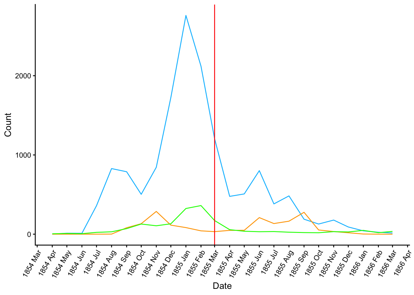
nightingale_df <- Nightingale |> as_tibble()

nightingale_df |>
    ggplot() +
    geom_line(aes(x = Date, y = Disease), color = 'deepskyblue') +
    geom_line(aes(x = Date, y = Wounds), color = 'orange') + 
    geom_line(aes(x = Date, y = Other), color = 'green') +
    scale_x_date(date_breaks = 'month', date_labels = '%Y %b') +
    guides(x = guide_axis(angle = 60)) +
    geom_vline(xintercept = ymd('1855-03-01'), colour = "red") +
    labs(y = 'Count') +
    theme_classic()

Public Library Survey 2010: Book Mobiles

# bk_df